I’m going to build predictive solar wind computational model using Particle burst engine and estimate its parameters.
Model and its parameters
The model has the following parametres:
- D – Distance between the Earth and the Sun
- Vel(a) – function of coronal hole area that calculates burst velocity
- Den(a) – function of coronal hole area that calculates burst density
- Vb – background wind velocity
- Db – background wind density
- Sigma – standard deviation of normally distributed fluctuation around estimated velocity mean
The overall average solar wind velocity at arbitrary distance from the Sun (x) at arbitrary time moment (t) is the following.
[latex]\displaystyle V(x,t) = \frac{V_b D_b + \sum_i V_i D_i I(i,x,t)}{D_b + \sum_i D_i I(i,x,t)}[/latex]
Where
$latex V_i=Vel(a_i) $ is velocity of i-th particle burst generated by i-th coronal hole.
$latex D_i=Den(a_i) $ is density of i-th particle burst generated by i-th coronal hole
[latex]
I(i,x,t) = \begin{cases} 1, & \mbox{if particle burst } i\mbox{ is at location }x\mbox{ at time moment }t \\ 0, & \mbox{otherwise} \end{cases}
[/latex]
Indicator function that chooses only particle burst that are at right location at right time moment.
Computational experiment
Assumptions
For this computational experiment I fitted 2nd order ascending polynomial functions as Vel(a) and Den(a)
The model time resolution is one minute. Thus 1 model time tick is 1 minute of real time.
The model space resolution is 1.0×10⁸m. 1 model space step (bin) is 1.0×10⁸m which is approximately 10 Earth diameters, and 1 AU is ~ 1500 model space steps.
The maximum coronal hole relative area can be 20% of the visible Sun area.
The maximum solar wind burst velocity considered to be 1 bin per 1 tick which is 1.0×10⁸m per minute which is 1666.(6) km/s.
Data used
As coronal hole area data used to emit bursts I used continuous subset of observations of 2015 year (between 40 to 8000 hours from the beginning of 2015 year, which is about 2 January 2015 – 30 November 2015)
Reference observations of solar wind velocity start little bit later to wait until first bursts reach the Earth. Thus references observations are per hour observations of 2015 year (between 150 and 8000 hours from the beginning of the year, which is about 7 January 2015 – 30 November 2015)
I consider that 5 days since the first bursts are emitted is enough to establish continuous flow of bursts at Earth distance.
Experiment
I did several runs of model parameter fitting using MCMC fitter developed in MSR Cambridge in collaboration with our lab.
I will evaluate 5 parameter sets that gave the maximum likelihood of observed values (MLE).
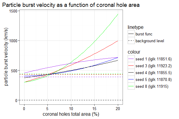
The following figure demonstrates five fitted functions of velocities that give maximum likelihood.
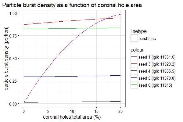
Corresponding fitted burst density function are
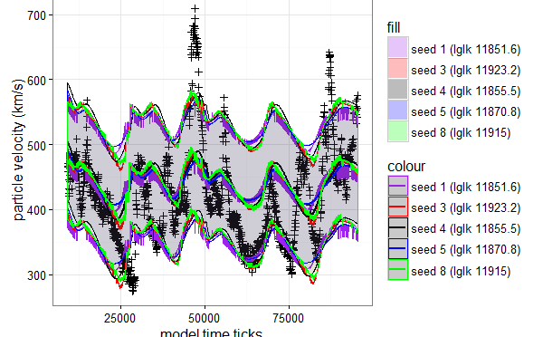
If we draw simulations using the functions above we get
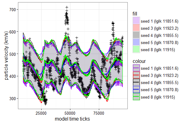
Crosses indicate real observations of the solar wind velocities.
Solid lines of difference colours represent the estimated mean solar wind velocities. Shaded areas represents mean +/- 1 noise sigma intervals.
Conclusions
As a result, even without explicit evaluation of error rates it can be seen that solar wind computational model behaves poorly for now. Simulated solar wind varies significantly less in magnitude than real wind measurements.
It can indicate that the model miss some important features. It stops the fitter to reduce noise and fit the variability better.
I can foresee the following causes of poor fitting:
- To strict “denoise” of coronal area predictor
- Circular approximation of Earth orbit instead of elliptical (parameter D)
You can reproduce the experiment using docker: “docker run -d -e seed=1 dgrechka/solarwindmodelfitter:0.3”
In addition the latest docker image of the fitter is here.
R report for figures generation.
This is a part of large solar wind prediction experiment, which I describe in a separate post.