The problem
There is a coldproof box with electronics (e.g. smart house control center).
We need to detect any environmental anomalies inside the box-case like overheating, coldproof failure or any other.
The plan
- The first thing to do is to gather some measurements data of normal system operation.
- Define a probabilistic model of normal operation.
-
Infer the parameters of the model with respect to the gathered measurements.
At this point we get the ability to evaluate the likelihood of every single measurement by substitution the measurement values vector to the probability density function of the modeled multivariate variable.
- Choose the likelihood threshold value to be able to distinguish between normal and anomaly system state.
When the likelihood value crosses the threshold (the measurement is too unlikely) we can admit that the system is in an anomaly state.
How to choose the threshold?- Well, Andrew Ng proposes to manually label several anomaly points.
- After we have reference positive (anomaly) and negative (normal operation) samples we can define an optimization problem that maximizes some classification score (e.g. F1-score). The classification threshold value is a parameter to optimize in this case.
- Perform the optimization with respect to the validation data.
- Measure the performance of the model (e.g. the same F1-score) on some additional test set.
Gathering the data
I recorded per minute measurements of air temperature and relative humidity sensors inside the box for 40 consequent days. This is about 60000 data points.
Do all of the recorded values correspond to normal operation?
I set the experiment of the accident (considered to be anomaly): the coldproof cover is not locked, so the cold out of the box air can flow inside the box
This is how the drop in temperature time series look like.

The red points reflect the box-opened case. While the black ones reflect the closed cover.
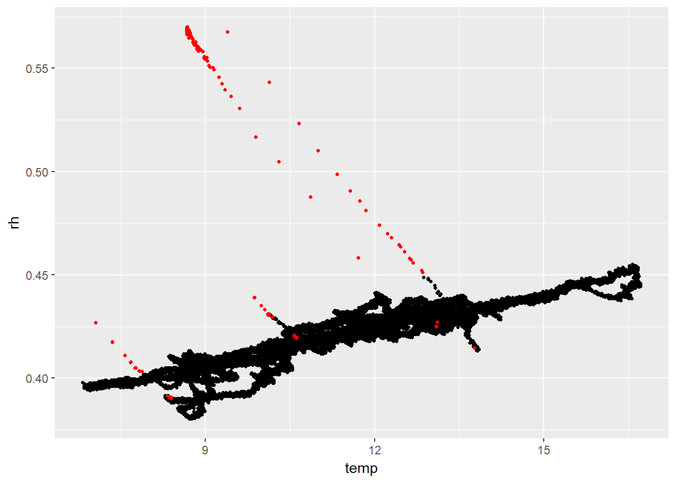
If we plot the same set of red points along with all other ~60 000 points on Temperature/RelHum plane we can see the following:

What we actually see is that in case of an accident, the drop in air temperature with the same amount of moisture in the air results in increase of relative humidity.
This picture suggests the following hypothesis: the event of box-case closure failure comes along with negatively correlated set of points.
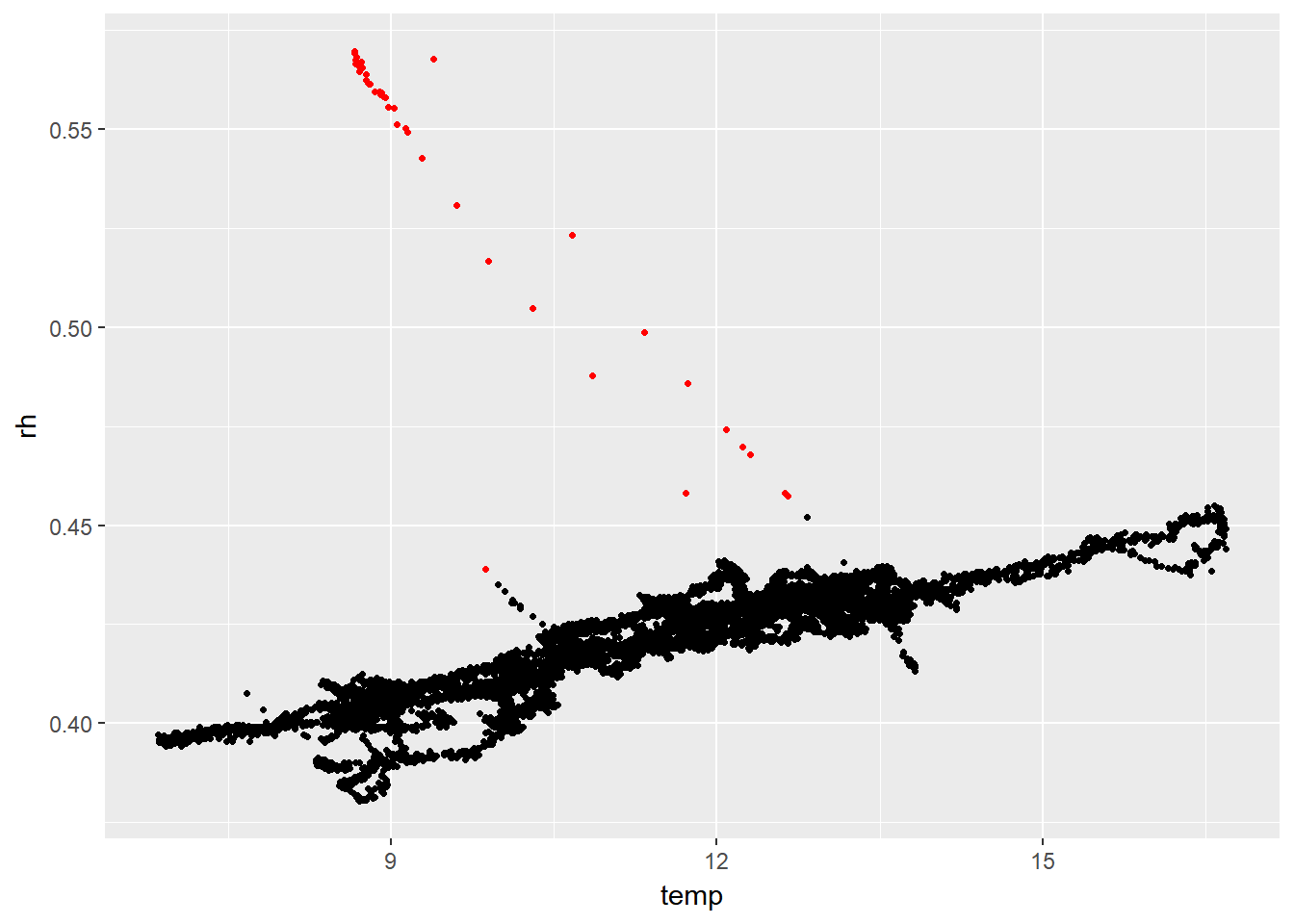
If we mark a series of negatively correlated points as anomaly (calculating correlation inside running window over time-series) we get the following:
The model and parameter inference
The density of observed measurements does not look like any well known distribution


Rather it looks like mixed set of normal distributions (with several peeks)
However, the correlation between air temperature and relative air humidity is strong during normal operation. Pearson correlation is 0.91!
That’s why ignoring correlation would be too rough. We need to model observed measurements as a multivariate variable,
This simplest variant is multivariate normal (Even though separately the distributions are not quite normal).
Multivariate normal distribution is parametrized with means vector and covariance matrix.
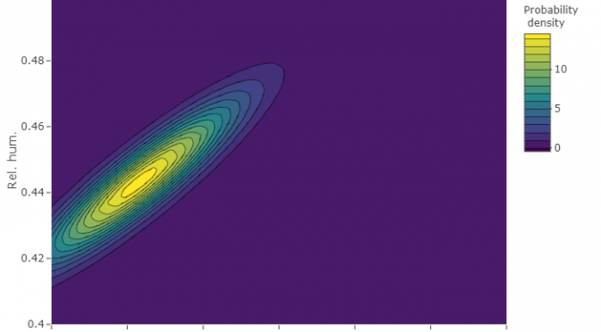
After calculating these parameters and plotting the density function we get the following.


The black curve here is kde while the red one is normal distribution model.
Although the separate plots above (temperature and rel. humidity) show that the model does not fit real density very well, joint probability distribution is well shaped. Just as a set of measurement points presented in above plots!

The threshold for anomaly
There are 57200 non-anomaly points and 147 hand-labeled anomaly points (see plots with red and black points above) in total in our disposal. I split the data as follows.
All non-anomaly points are split into training, validation and test sets in 60% / 20% / 20% ratio.
Anomaly points are split into validation and tests sets in 50% / 50% ratio.
Training set (containing only non-anomaly points) has already been used in the previous section when we chose the means vector and the covariance matrix for the multivariate distribution.
Now we use validation set (11440 non-anomaly and 74 anomaly points) to infer the threshold (epsilon) for flagging a measurement as anomaly. As the anomaly points count is much less then non-anomaly (as it should be in every anomaly detection system :-) ) it is wise to use F-measure to score the performance of classification. We will use the F1.
Optimisation run achieved a F1-score of 0.756. It corresponds to the density value of 0.00089. Everything is ready now for the operation of the anomaly detection. If measured temperature and humidity substituted into density function is less then 0.00089 we consider this as anomaly.
Performance test
Now it is time to use the third dataset, a test dataset.
We will evaluate how the model performs of the previously unseen testset. The results are:
## Confusion Matrix and Statistics

##

##           Reference

## Prediction  anom  norm

##       anom    47     0

##       norm    26 11440

##

##                Accuracy : 0.9977

##                  95% CI : (0.9967, 0.9985)

##     No Information Rate : 0.9937

##     P-Value [Acc > NIR] : 1.912e-10

##

##                   Kappa : 0.7823

##  Mcnemar's Test P-Value : 9.443e-07

##

##             Sensitivity : 0.643836

##             Specificity : 1.000000

##          Pos Pred Value : 1.000000

##          Neg Pred Value : 0.997732

##              Prevalence : 0.006341

##          Detection Rate : 0.004082

##    Detection Prevalence : 0.004082

##       Balanced Accuracy : 0.821918

##

##        'Positive' Class : anom
This corresponds to F1 = 0.783
The prediction looks like this:
Good!
The anomaly detection system is ready.