Intro
The Solar Wind Particle Burst Engine models the solar wind by simulating bursts of particles emitted by coronal holes. The idea is to simulate continuous flow of particles using discrete representation of the world. We can represent the wind as a finite number of particle bursts. The world space is one dimensional. It is represented with finite number of bins. The bins are enumerated with index. Greater the index, greater the distance of the bin from the Sun. Therefore the bin with index 0 corresponds to the Sun surface. Each bin at every particular time moment can “contain” zero or more particle bursts. At every world time tick (the time is modelled in a discrete way in form of integer ticks) the particle bursts move out of the Sun by leaving one bin and getting into another.
Since we can characterise each burst with some emergence time (tick) and some velocity, each simulation run can be entirely described as a set of bursts. The velocity of every burst is constant, we consider it as a function of coronal holes at the burst emergence time moment.
Demo
Here you can see the demo run of burst engine:
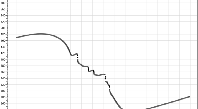
Three standalone bursts are emitted at 0, 10 and 20 simulation ticks with corresponding velocities of 0.2, 0.5 and 1.0 bin/tick.
The Y axis shows the average velocity of all the bursts in the bin.
In addition, this simulation can also be represented as burst “traces”:
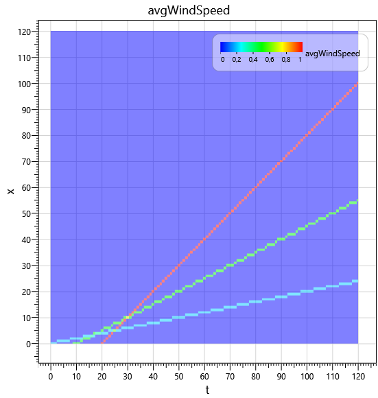
The colour of this colormap reflects the average velocity of all bursts at space-time point.
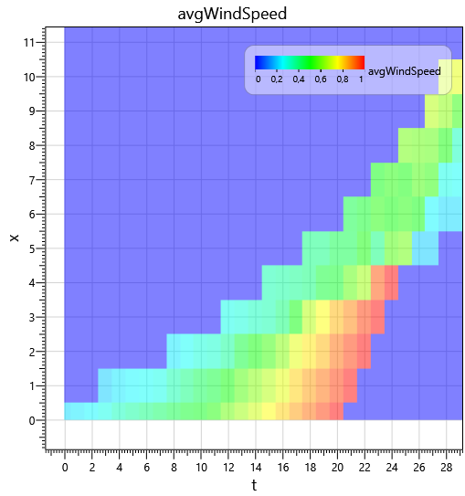
Furthermore, if we emit a burst at every simulation tick we can model the continuous flow of the solar wind. The only requirement here is not to have velocity exceeding 1.0 bin/tick. To emit the burst at every tick we can interpolate the properties of closest bursts. Hence, for the example above we can get the following “continuous” solar wind flow (20 bursts acquired from linear interpolation of 3 standalone bursts).
The traces for this configuration now look like this:
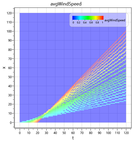
We can see that discrete nature of the model is exposed in the late steps (50 and greater). This happens because there are nor more bursts are emitted after final burst at tick 20.
Looking at ticks interval 0 to 20 we can see that the simulated wind is “continuous” (e.g. without sudden drops of average velocity to zero)
Feeding simulator with real data
As a result, we can construct the simulation run by advancing the model world induced by evaluation of real coronal holes. For example, for year 2015 the wind can be modelled like:
Trace view in this case transforms from “traces” into a velocity magnitude “field”:
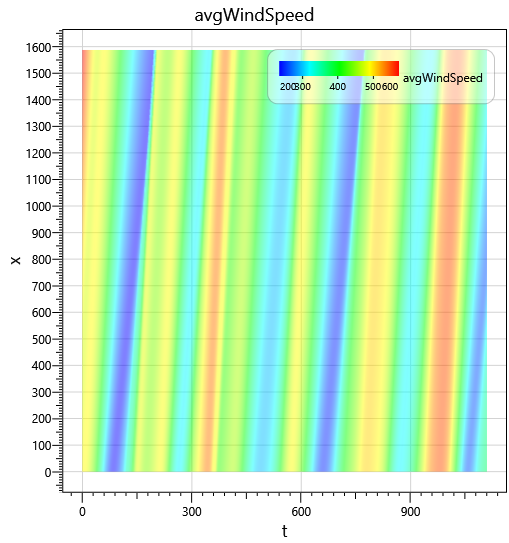
You can notice that most of the time the flow indeed looks like continuous. Sometimes the flow scrambles (e.g. see time moment around tick 9150) which indicates that the way in which I design the engine can be not well suited for modelling real world.
I will discuss the burst velocity function of coronal holes, space bin sizes, model tick length as well as converting velocity units from real world to model and vise versa in additional post where I perform inference of most of these parameters.
This is a part of large solar wind prediction experiment, which I describe in a separate post.